Velocity, acceleration and jerk

Introduction

The Newton $F=ma$ force rule states that force and acceleration are proportionally related. Is it possible to accelerate without noticing the jerk? The method is used in elevators, for example, and hopefully in modern (electric) cars.

We consider the acceleration the robot is subjected to while accelerating it using different acceleration functions. We use Vernier ACC-BTA (25g) sensor with both NXT Adapter and Labquest, but you may use the accelerometer of your mobile phone, also.

Robot

Almost any robot will be ok, we use Asimov 2/ Verne.

Sensor

The Vernier acceleration sensor (MBA-ACC, 25g) with the NXT Adapter is used. The sensor is attached to port number 4.

Very simple test program to see what are the measured values is shown below. The values are in arbitrary scale, and need to be normalized. We found, that the

#!/usr/bin/env python3
# https://sites.google.com/site/ev3devpython/

from ev3dev2.sensor import *
from ev3dev2.sensor import INPUT_4

import time
import os

os.system('setfont Lat15-TerminusBold32x16')  # Try this larger font

p = Sensor( INPUT_4 )
p.mode="ANALOG-1"

def measureAcc(p):
    acc = p.value(0)
    return acc

tstep = 0.001

while True:
    acc = measureAcc(p)
    print( acc )
    time.sleep( tstep )

Theory

The time derivative of position is velocity, then we have acceleration, and the derivative of acceleration is called jerk, $j$. ${\frac {da}{dt}}=j$ Then we have snap, crackle and pop.

See the Wikipedia page on the physiological_effects of jerk. Anyway, there might be jerky rides.

We measure the acceleration of robot, and use a numerical differential method to estimate the jerk. We use the symmetric differential;

$j(t)={\frac {da}{dt}}={\frac {f(t-h)+f(t+h)}{2h}}$ in which the first-order error cancels, and the error is $-{\frac {1}{6}}f^{(3)}(x)h^{2}$ where $t-h<x<t+h$.

We will start from zero to $t_{0}=5000$ ms where the speed should be at maximum value, $L=100$.

Standard Scheme

The ev3dev Python standard scheme is . . .

Linear acceleration

The Linear Acceleration

$v(t)={\begin{cases}{\frac {L}{t_{0}}}t&&{\text{if }}t<t_{0}\\L&&{\text{if }}t\geq t_{0}\end{cases}}$

because the continuity constraint $at_{0}=L$ gives that $a=L/t_{0}$. The graph is shown on Desmos .

Sinusoidal acceleration

Sine acceleration

The sine curve is a harmonic motion between -1 and 1 with period $2\pi$. We use only one period, and scale that to correct acceleration function. The sine accelerates rather smoothly.

$v(t)={\begin{cases}{\frac {L}{2}}(\sin({\frac {\pi }{t_{0}}}t-{\frac {\pi }{2}})+1)&&{\text{if }}t<t_{0}\\L&&{\text{if }}t\geq t_{0}\end{cases}}$

See the interactive Desmos graph.

Logistic Curve

The logistic Curve with parameters.

A logistic function is S-shaped curve (or sigmoid curve) is a function with equation

$v(t)={\begin{cases}v(t)={\frac {L}{1+e^{-k(t-t_{0})}}}&&{\text{if }}t<t_{0}\\L&&{\text{if }}t\geq t_{0}\end{cases}}$

where $t_{0}$ is the $t$ value of the sigmoid's midpoint, $L$ is the curve's maximum value and $k$ is the curve's growth rate. See the Desmos graph.

The bumb function

The Bumb Function.

There exists some well-known every-where differentiable functions, with a compact support. One example is

$v_{1}(t)={\begin{cases}1&&{\text{if }}-a<t<a\\e^{-{\frac {(|t|-a)^{2}}{4a^{2}-t^{2}}}}&&{\text{if }}a\leq |t|\\0&&{\text{if }}t>2a\end{cases}}$

with $v(t)=100v_{1}(t-180)$. This is an example of a $C^{\infty }$ with support in $a-r\leq t\leq a+r$. We are going to take half of the curve to be our velocity function. The graph is shown on Desmos page.

See more about the function at Math Stack Exchange, and the references therein.

Example Codes

First, we use Python on computer to check the scripts of the acceleration functions. These functions are applied in the motor control part. The robot script logs the data, and the data is uploaded to the computer and analyzed later.

Python

The scripts are on a separate file called accFunction.py, which can be read in both scripts: on a computer and on a motor, to ensure the consistency.

import math

def vlin(t):
    L = 100
    t0= 5000
    if t > t0:
        return L
    if t < 0:
        return 0
    return L*t/t0

def vsin(t):
    L = 100
    t0= 5000
    if t > t0:
        return L
    if t < 0:
        return 0
    return L/2*( math.sin(3.14159*t/t0-3.14159/2)+1)
    
def vlog(t):
    L = 100
    t0= 5000
    if t > t0:
        return L
    if t < 0:
        return 0
    return L/(1 + math.exp(-0.00322*(t-2500)))

def vbum(t):
    L = 100
    a = 4600
    t1= 9270
    if t > a:
        return L
    if t < 100:
        return 0
    else:
        return L*math.exp(-((t1-t)-a)**2/(4*a**2 - (t-t1)**2) )

The velocity functions can be plotted using the following short script. The both files need to be in the same directory.

import matplotlib.pyplot as plt
import numpy as np
import accFunction 

t = np.linspace(-1000,3000,1000)

v = np.array([accFunction.vlin(ti) for ti in t])

plt.plot( t,v )
plt.xlabel('Time [ms]')
plt.ylabel('Speed')

Ev3dev

The robot program code is still for a second, and then starts accelerating according to the velocity function. The recorded accelerations are logged into corresponding log files, and the next run is appended at the end of the file.

Note that while pressing F5, the VS Code downloads the directory to the robot, and thus you might overwrite the log files. You may run the script from the brick or upload the log files to the computer in between, or you can upload the log files in a different directory.

#!/usr/bin/env python3
# https://sites.google.com/site/ev3devpython/

from ev3dev2.sensor import *
from ev3dev2.sensor import INPUT_4
from ev3dev2.motor import MoveSteering, OUTPUT_B, OUTPUT_C

import time
import os
import csv 

import math
import accFunction 

def measureAcc(p):
    acc = p.value(0)
    return acc

acc = accFunction.vlin
acc = accFunction.vsin
acc = accFunction.vlog
acc = accFunction.vbum

f = open(acc.__name__ + ".csv","a")
writer = csv.writer(f) 

steer_pair = MoveSteering(OUTPUT_B, OUTPUT_C)
p = Sensor( INPUT_4 )
p.mode="ANALOG-1"

s0 = time.time()*1000.0+1000 #One second pause before starting
while time.time()*1000.0 - s0 < 7000:
    t = time.time()*1000.0 - s0
    vt = acc(t)

    steer_pair.on(steering=0, speed=-vt)
    writer.writerow((time.time(), measureAcc(p) ))

f.close()

Analysis and Analysis Scripts

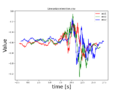
You can use almost any data analysis software, e.g. Geogebra or spreadsheet. The data on different runs is written after each other, and you might need to separate those by hand. We use a simple Python Pandas script, which is described at page Plot the acceleration. The data show on the images is smoothed using moving average of window size 50.

• 

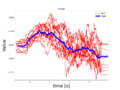
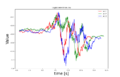
  Acceleration from about 10 runs using NXT Adapter

• 

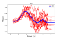
  Acceleration from about 10 runs using NXT Adapter

• 

  Acceleration from about 10 runs using NXT Adapter

• 

  Acceleration from about 10 runs using NXT Adapter

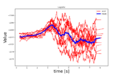
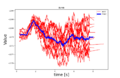
Because the data is such bumby, we checked the acceleration using Vernier Labquest. The data is qualitative similar to those above. Also, the LabQuest data is smoothed using the same window of 50 time steps.

• 

  Acceleration from 3 runs using LabQuest

• 

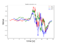
  Acceleration from 3 runs using LabQuest

• 

  Acceleration from 3 runs using LabQuest

• 

  Acceleration from 3 runs using LabQuest

The images are below.

Issues

The Vernier 25g accelerometer is not sensitive enough to give the possibility to integrate velocity or position.

Actually, we find the jerk cannot be estimated using this sensor.

Exercises

• Compare the measured acceleration values to those differentiated from the analytical speed functions. What do you observe?
• Use smaller t0, e.g. 2 seconds or 1 second to accelerate more rapid.
• The motor runs at high speed even though the steering speed is not 100. Change the maximum value L to some smaller, e.g. L=80. Compare, how this affects.
• The data is not calibrated, but it is easy to calibrate because the gravitational acceleration is $g=9.81m/s^{2}$. Thus, flip the robot on its nose, then on its neck, and you have two data points to calibrate on.
• Use the velocity function to integrate distance (use geogebra, or any other symbolic math program if you wish).
• Change the script to run on a given distance instead of a time. Use the distance functions given above. Draw a line on floor and use color sensor to check the measurements and accuracy.

Back to Mahtavaa Matematiikkaa 2020